What does impact body performance? | A machine learning approach

Data analysis with Pandas, data visualization with Seaborn and machine learning with Scikit Learn regarding a body performance features | Age, weight, body fat...
Published on December 22, 2021 by Andrés Ingelmo Poveda
jupyter notebook python data analysis pandas seaborn data visualization machine learning scikit learn
15 min READ
What does impact body performance? This is the question a lot of us have asked themselves sometime. Am I going to perform better if I’m lighter? What if I’m taller?
In this blog post, I will take a machine learning approach to analyse more than 13,000 observations from individuals aged between 20 and 64 years and its results in different performance tests depending on their height and weight among other variables.
The final objective of the analysis is to perform some unsupervised learning to discover possible clusters with common characteristics and a linear regression to estimate what are the most important features that define each result.
Data cleaning
The dataset was already clean. However, a few modifications needed to be done. Because I don’t want to spend a lot ot time here, you can check the steps I took to clean it on my Kaggle notebook or my GitHub project.
Data exploration
The first 5 rows of the cleaned dataset follows the next structure:
| age | gender | height_cm | weight_kg | body fat_% | diastolic | systolic | gripForce | sit and bend forward_cm | sit-ups counts | broad jump_cm | class | lean_BMI | |
|---|---|---|---|---|---|---|---|---|---|---|---|---|---|
| 0 | 27 | M | 172.3 | 75.24 | 21.3 | 80 | 130 | 54.9 | 18.4 | 60 | 217 | C | 19.9459 |
| 1 | 25 | M | 165 | 55.8 | 15.7 | 77 | 126 | 36.4 | 16.3 | 53 | 229 | A | 17.278 |
| 2 | 31 | M | 179.6 | 78 | 20.1 | 92 | 152 | 44.8 | 12 | 49 | 181 | C | 19.321 |
| 3 | 32 | M | 174.5 | 71.1 | 18.4 | 76 | 147 | 41.4 | 15.2 | 53 | 219 | B | 19.0532 |
| 4 | 28 | M | 173.8 | 67.7 | 17.1 | 70 | 127 | 43.5 | 27.1 | 45 | 217 | B | 18.5799 |
I usually like to follow my analysis by plotting the histogram and the correlation matrix to extract some insights from the data:
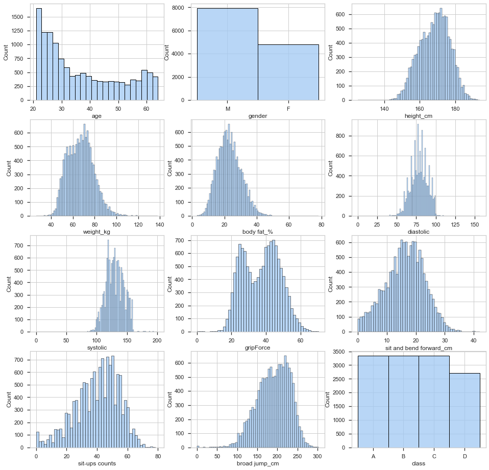
From this visualization we can say that there are two features that are not normally distributed: the age and the gender. There are more males than females in the dataset and more young than old people. Other than that, the other features are pretty evenly distributed.

This correlation matrix show some interesting data. For example, it seems to be a strong negative correlation between body fat and the broad jump test results. This means that, the more body fat, the worst the result in this test is. Another insight we can get is that weight is positive correlated to weight, meaning more height, more weight, but body fat is negatively correlated. This means that taller people have usually a lower body fat percentage.
Data preprocessing
After performing some superficial data analysis, it is time to prepare our dataset to use it in machine learning purposes. In this step, I will encode the categorical variables and standardize the features. You can check the steps I took on my Kaggle notebook or my GitHub project.
The scaled dataset looks like this:
| age | gender | height_cm | weight_kg | body fat_% | diastolic | systolic | gripForce | sit and bend forward_cm | sit-ups counts | broad jump_cm | class | lean_BMI | |
|---|---|---|---|---|---|---|---|---|---|---|---|---|---|
| 0 | -0.709833 | 0.770644 | 0.454339 | 0.686597 | -0.236497 | 0.114976 | -0.015168 | 1.67392 | 0.318338 | 1.41688 | 0.653997 | 0.542015 | 0.793553 |
| 1 | -0.857298 | 0.770644 | -0.417975 | -0.966094 | -1.02083 | -0.165797 | -0.28817 | -0.0684791 | 0.00181325 | 0.907212 | 0.962995 | -1.29698 | -0.331118 |
| 2 | -0.414904 | 0.770644 | 1.32665 | 0.921238 | -0.404569 | 1.23807 | 1.48634 | 0.722665 | -0.64631 | 0.615971 | -0.272998 | 0.542015 | 0.530114 |
| 3 | -0.341171 | 0.770644 | 0.717228 | 0.334635 | -0.642671 | -0.259388 | 1.14509 | 0.40244 | -0.163986 | 0.907212 | 0.705497 | -0.377481 | 0.417254 |
| 4 | -0.636101 | 0.770644 | 0.633581 | 0.045584 | -0.824749 | -0.820934 | -0.219919 | 0.600226 | 1.62966 | 0.324729 | 0.653997 | -0.377481 | 0.217715 |
I also thought it would be good to perform some dimensionality reduction. In this dataset, there are a lot of features that influence in the final classifications. The higher number of features, the harder it is to work with. As many of these features are correlated, they are redundant.
I will use the Principal Component Analysis (PCA) to reduce the dimensions.
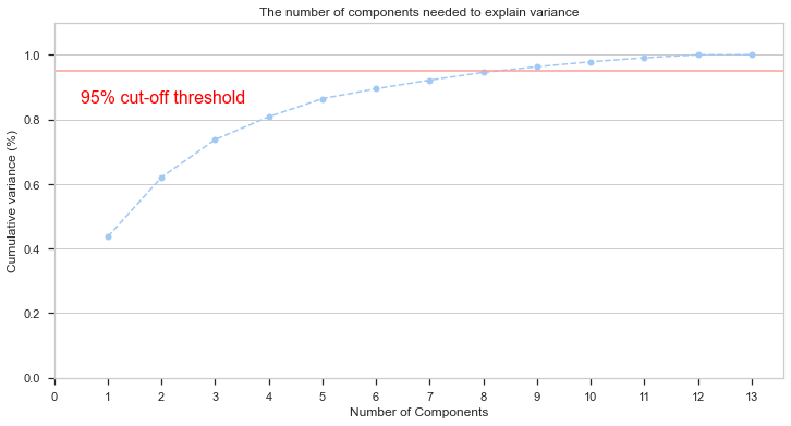
The above chart shows that, to achieve a 95% of variance explained, we need to get at least 8 variables.
Clustering
Once the dimensionality reduction is done, we’ll move to clustering. The clustering technique I’m going to use is the Agglomerative Clustering. This type of clustering is a hierarchical clustering method that involves merging examples until the desired number of clusters is achieved.
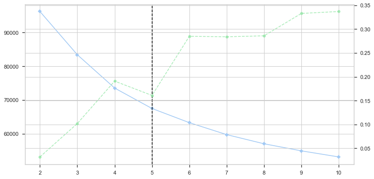
The chart above indicates that the optimal number of clusters for this dataset is 5. After performing Agglomerative Clustering and parsing the data into the original dataset, it looks like this:
| age | gender | height_cm | weight_kg | body fat_% | diastolic | systolic | gripForce | sit and bend forward_cm | sit-ups counts | broad jump_cm | class | lean_BMI | clusters | |
|---|---|---|---|---|---|---|---|---|---|---|---|---|---|---|
| 0 | 27 | M | 172.3 | 75.24 | 21.3 | 80 | 130 | 54.9 | 18.4 | 60 | 217 | C | 19.9459 | 0 |
| 1 | 25 | M | 165 | 55.8 | 15.7 | 77 | 126 | 36.4 | 16.3 | 53 | 229 | A | 17.278 | 0 |
| 2 | 31 | M | 179.6 | 78 | 20.1 | 92 | 152 | 44.8 | 12 | 49 | 181 | C | 19.321 | 0 |
| 3 | 32 | M | 174.5 | 71.1 | 18.4 | 76 | 147 | 41.4 | 15.2 | 53 | 219 | B | 19.0532 | 0 |
| 4 | 28 | M | 173.8 | 67.7 | 17.1 | 70 | 127 | 43.5 | 27.1 | 45 | 217 | B | 18.5799 | 0 |
Evaluating models
Since this is an unsupervised machine learning model, we don´t have a tagged feature to evaluate our model. The purpose of this section is to study the patterns in the clusters formed an determine the nature of the clusters’ patterns.
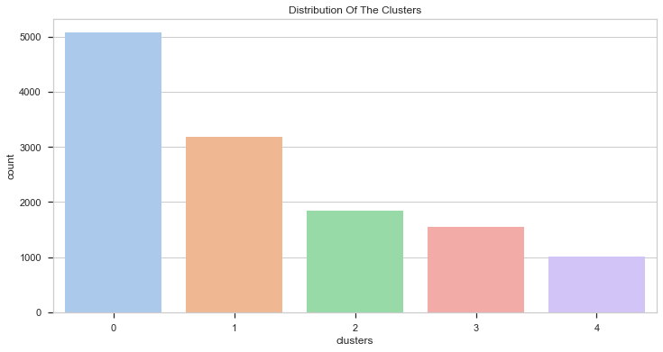
As we can see in the above chart, the clusters are not equally distributed. Let’s try to figure out what each one can mean. First thing I’m going to do is check if height and weight has something to do with the score.
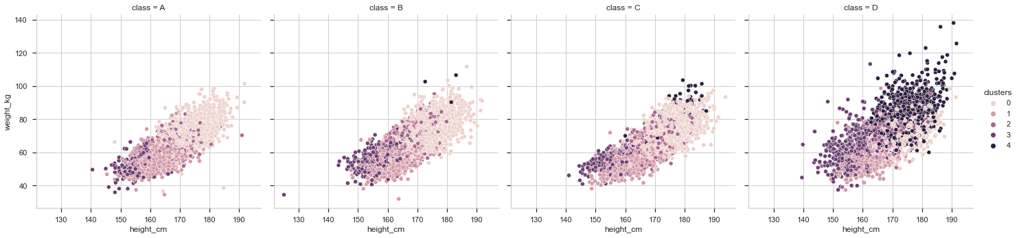
It is pretty clear that there is a correlation between height, weight and score. The individuals who weighted more, scored the worst in the test on average. We can also see that majority of cluster 4 observations are in the class D. Let’s get more details on this.
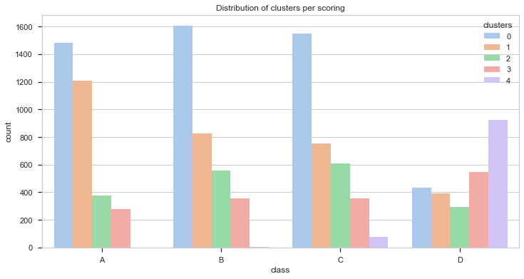
The chart above doesn’t provide much information we didn’t know before. Cluster 4 is related with people with the worst score. However, the other three clusters are distributed evenly between the other three scores. It has to have another meaning.
Profiling
In this section, I will try to deduce which individuals are in which cluster. To decide that, I will be plotting some of the features present in the dataset.
Let’s first analyse the relation between weight and the score on different tests:
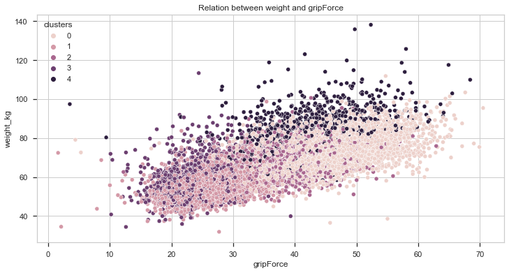
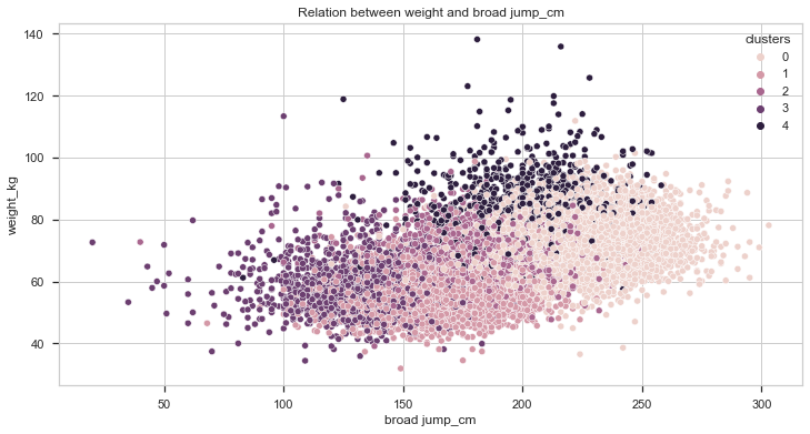
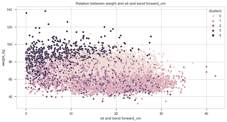
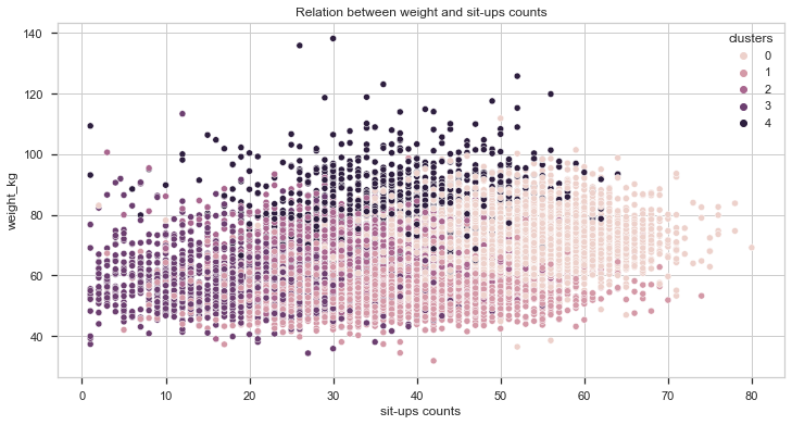
Taking a look at the charts plotted we can say that cluster 4 individuals are heavier, on average, than the other individuals. It is also important to notice that, the heavier the individual, the better gripForce score. In the the sit-ups and broad jump tests, it seems to be a positive correlation between weight and better results but it is not as high as the previous one.
Let’s see know how the height compares to the score.
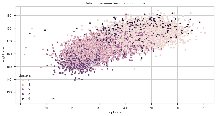
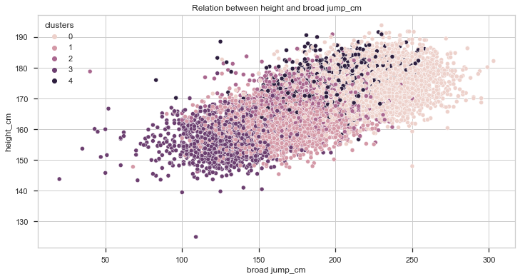
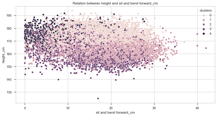
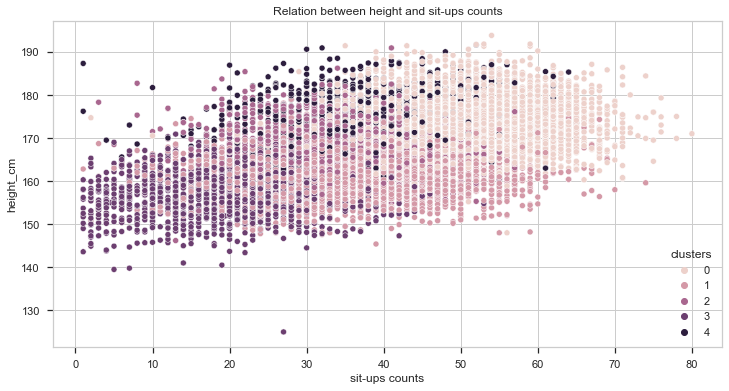
With this plot we can get some interesting insights!
- It seems that taller people perform better in broad jump and grip force tests. However, in the other two, height doesn’t seem to provide any advantage at all.
- Individuals from cluster 0 are taller than the average while individuals from cluster 3 are shorter.
Now, let’s compare the results with the age.
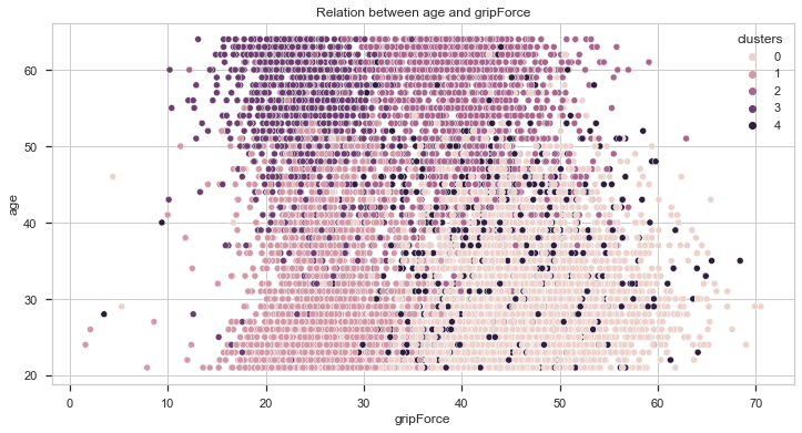
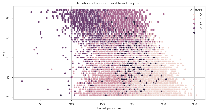
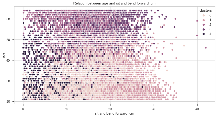
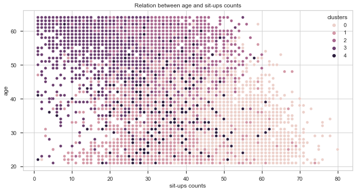
From the above charts, we can also get two important insights:
- The younger the individual, the better the score.
- Individuals from clusters 2 and 3 are, on average, older than the rest of the dataset.
Let’s compare it now with the lean BMI.
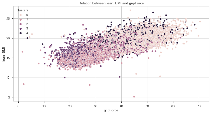
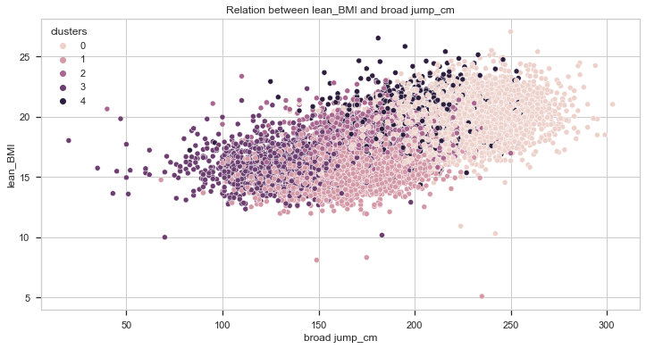
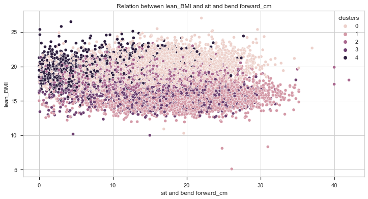
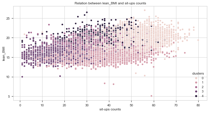
From the charts above, we can also get two important insights:
- Individuals with higher lean BMI performed better in strength tests (grip force and broad jump).
- Individuals from cluster 0 have the highest lean BMI while individuals from cluster 1 have the lowest.
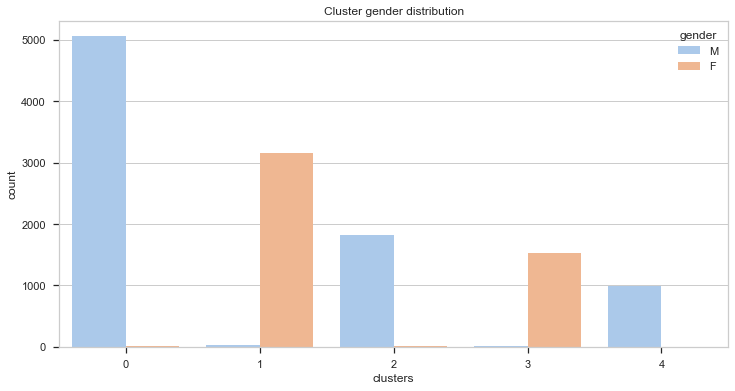
Before trying to get more detailed information to profile each cluster, let’s get the gender distribution for each one.
Now, let’s group all observations by cluster type and get the mean of all the features to get more details regarding each cluster.
| clusters | age | height_cm | weight_kg | body fat_% | diastolic | systolic | gripForce | sit and bend forward_cm | sit-ups counts | broad jump_cm | lean_BMI |
|---|---|---|---|---|---|---|---|---|---|---|---|
| 0 | 29.7555 | 174.261 | 72.9637 | 17.8405 | 78.6195 | 131.545 | 45.3652 | 15.9044 | 51.2011 | 225.307 | 19.6739 |
| 1 | 29.5054 | 162.187 | 56.051 | 26.59 | 74.3606 | 120.725 | 26.7833 | 20.4487 | 37.5047 | 166.169 | 15.5609 |
| 2 | 54.924 | 169.396 | 69.0541 | 21.6944 | 83.4058 | 138.102 | 39.8659 | 13.3849 | 34.7137 | 187.094 | 18.7648 |
| 3 | 53.7969 | 157.224 | 58.085 | 31.6835 | 78.1181 | 130.494 | 24.3199 | 17.5218 | 20.2031 | 132.638 | 15.9078 |
| 4 | 33.952 | 175.025 | 83.541 | 26.6361 | 86.0193 | 138.744 | 42.8916 | 8.46951 | 38.1858 | 200.612 | 19.874 |
Now we can draw some conclusions to determine which type of people form each cluster:
- Cluster 0: young tall males with high lean BMI.
- Cluster 1: young small females with low lean BMI.
- Cluster 2: old tall males with high lean BMI.
- Cluster 3: old small females with low lean BMI.
- Cluster 4: overweight males in its majority.
Linear Regression
At this point of the analysis, I thought it would be good to know what features determine the test results. For example, is a heavier person going to perform better in a strength test? To answer these kind of questions, I’m going to run a linear regression model.
I builded four different models: grip force, sit and bend forward, sit-ups count and broad jump. Again, you can check more information regarding the steps taken for linear regression on my Kaggle notebook or my GitHub project. The score for each model is as following:
The score for model gripForce is:  0.7744484932198941
The score for model sit and bend forward_cm is:  0.24417579569506664
The score for model sit-ups counts is:  0.616084673391197
The score for model broad jump_cm is:  0.7425962295683317
Then, I plotted the coefficients to check which one was making more differences within model. In other words, I wanted to know which feature contributed the most in a positive or negative way to the test score.
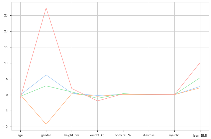
As we can see in the above graph, the most influential parameter in all test is the gender. It looks like male individuals perform better than female in strength tests while women do better in flexibility ones. The second most important parameter is the lean BMI and it makes sense. The higher the lean BMI is, the lower the body fat is, the higher the muscle mass is, the better an individual can perform in physical tests. Height and weight are somewhat important and came make a different depending on the test. For example, a heavier guy is probably going to perform worse on the broad jump and better in the grip force than a lighter one.
At this point, we know that gender plays a huge rol in explaining the test result. Let’s remove this bias and try it again.
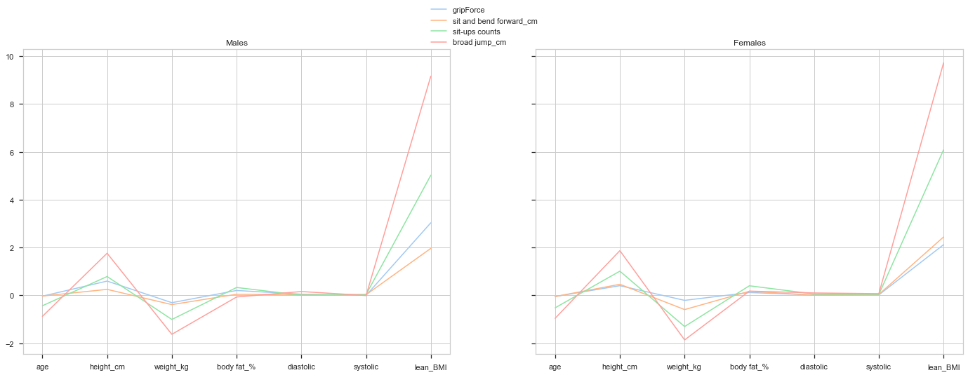
Both plots show similar results. Height influence positively in all results while weight does it negatively. This means that the taller an individual is, the better he is going to perform and, the heavier, the worse. Lean BMI seems to be the most influential variable af all and it makes sense. This variable measures the amount of muscle an individual has depending on his height. The higher the lean BMI is, the more athletic he is going to be, therefore, the better he is going to perform in physical tests.
Conclusions
The unsupervised clustering provided a good data segmentation. Despite this technique wasn’t really needed to carry on the analysis, it showed five different groups with common characteristics.
From the data analyzed, we can draw the conclusion that body performance decreases during the years and males and females have different strengths. In this case, females were more flexible while males did better in strength tests.
Also, a higher body fat can lead to bad body performance and higher blood pressure.